5. Getting Started with RIVET
The RIVET software consists of two separate but closely related executables: rivet_console, a command-line program, and rivet_GUI, a GUI application. rivet_console is the computational engine of RIVET; it implements the computation pipeline described in the previous section. rivet_GUI is responsible for RIVET’s visualizations and also provides a convenient graphical front-end to the functionality of rivet_console. Thanks to this front-end, RIVET’s visualizations can be carried out entirely from within rivet_GUI.
For new users looking to acquaint themselves with RIVET, we recommend starting by using rivet_GUI to explore RIVET’s visualization capabilities. In this section, we provide a simple introduction to running RIVET via rivet_GUI. Later sections of the documentation provide more detail on how to use rivet_console and rivet_GUI. Users who wish to use RIVET for purposes other than visualization (e.g. machine learning or statistics applications) will want to familiarize themselves with the command-line syntax of rivet_console, but we recommend all users read this introduction first.
5.1. Getting started with rivet_GUI
When the user runs rivet_GUI, the following window opens:
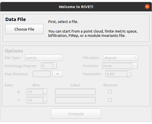
To start a computation, we first select a file by clicking the Choose File button. RIVET can handle several different types of input: Point clouds, finite metric spaces, simplicial bifiltrations, and short chain complexes. These file formats for these input types are discussed in detail in Input Data Files.
In this introduction, we consider just one simple type of input file, a CSV file specifying a point cloud in \(\mathbb{R}^n\). Each line of the file gives the \(n\) coordinates of one point; these coordinates are written as numbers separated by commas or white space.
We will use the file data/Test_Point_Clouds/circle_300pts_nofunction.csv from the RIVET repository. This file specifies 300 points in \(\mathbb{R}^2\). The first five lines of the file are as follows:
1.57,2.40
1.21,2.70
0.79,-2.44
-2.44,-2.24
-2.54,-1.25
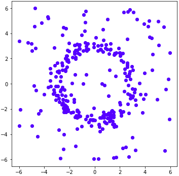
The 300 points in the file data/Test_Point_Clouds/circle_300pts_nofunction.csv form a noisy circle in \(\mathbb{R}^2\), as pictured below.
We will use RIVET to compute a ball density function \(\gamma\) on this data set, and construct the function-Rips bifiltration with respect to \(\gamma\). (See Function-Rips Bifiltration for the definitions of these terms.) The 1st persistent homology module of the function-Rips bifiltration of this data algebraically detects the presence of a “loop” in the data. Below, we illustrate how RIVET visualizes this persistence module.
Upon selecting a file, RIVET activates the input selectors in the Options panel of the dialog box. The following figure shows RIVET file input window, with the selection of options we will use in this example.
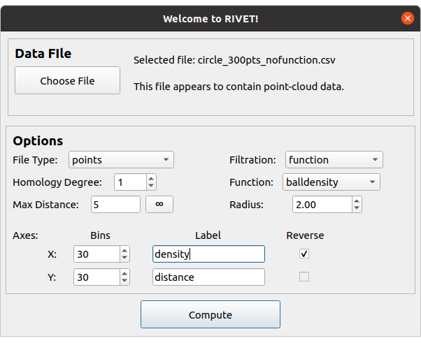
We now briefly discuss the available options.
The File Type selector tells RIVET what type of input file it should expect. For this data file, we must select the default option, points.
The Homology Degree selector chooses the degree of the homology module RIVET computes. (Currently, RIVET computes only a single degree of homology at a time. A user who wishes to examine homology in multiple degrees, e.g., in degrees 0 and 1, will need to run multiple RIVET computations on the same input data.) Since we want to discern a “loop” in the data, in this example we select homology degree 1.
The Max Distance selector specifies the maximum length of edges that RIVET will include in the bifiltration it constructs. This controls the size of the bifiltration, and thus the cost of the computation. We choose a max distance of 5 for our example. The max distance can be set to infinity, so that every possible edge appears in the bifiltration; this is done by typing “inf” or clicking on the button with an infinity symbol. The default max distance is infinity.
Three input selectors on the right side of the box determine what bifiltration RIVET will build from the point cloud. The Filtration selector offers two options: degree and function. The degree option builds a degree-Rips filtration, as described in Degree-Rips Bifiltration. Here, we choose the function option to build a function-Rips bifiltration.
The function-Rips bifiltration depends on the choice of a real-valued function on the point cloud, which is specified by the Function selector. Here, we choose the balldensity option, which specifies the function to be a ball density function. Other options for the function include a Gaussian density function, an eccentricity function, and a user-defined function, which must be specified in the input file; see Input Data Files for details.
The ball density function depends on a choice of radius parameter, which must be provided in the box below the Function selector. Here, we choose a radius of 2.
The selectors in the lower portion of the Options box deal with the coordinate axes. The Bins selectors specify the coarsening of the homology module, as described in Coarsening a Persistence Module. The number of bins is set separately for the x-axis and the y-axis. The coarsening controls the number of distinct bigrades where generators and relations of the module can appear. Thus, specifying a smaller number of bin values will speed the RIVET computation and reduce its memory, but will result in less accurate approximation to the uncoarsened homology module. In this example, we set both bin values to 30, though higher values could also be used without difficulty.
Next, the user may specify the Label for each axis in the RIVET visualization. For a function-Rips filtration, RIVET presents the function values along the x-axis. Since we are computing a density estimator, we enter “density” for the x-axis label. We keep the default “distance” label for the y-axis.
Lastly, the Reverse checkboxes allow the user to reverse axis directions. For example, when using a density function, we typically want points with larger density values to enter the bifiltration before points with smaller density values; thus, when we select the “balldensity” function, the Reverse box for the x-axis is checked by default. It is not possible to reverse the distance axis for a Rips filtration, so in this example, the y-axis Reverse selector is unavailable.
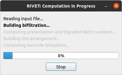
We now click Compute at the bottom of the file input window. This starts the RIVET computational pipeline, as described in Computation Pipeline. A progress box appears, as shown below.
5.2. Overview of the RIVET Visualization
When the computation finishes, RIVET displays the following visualization. This section gives a brief overview of the visualization elements; much more detail is found in The RIVET Visualization: Further Details.
The RIVET visualization contains two main windows, the Line Selection Window and the Persistence Diagram Window, shown in the screenshot below.
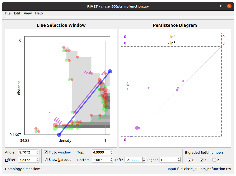
5.2.1. Line Selection Window
The Line Selection Window visualizes the Hilbert function values and the bigraded Betti numbers of a bipersistence module. In addition, it can interactively display the barcode obtained by restricting the module to an affine line. The viewable region is chosen as described in The RIVET Visualization: Further Details, and can be adjusted using the controls at the bottom of the window.
The Hilbert function is represented via grayscale shading of the viewable region, and points in the supports of \(\xi_0^M\), \(\xi_1^M\), and \(\xi_2^M\) are marked with translucent green, red, and yellow dots, respectively. The area of each dot is proportional to the corresponding function value. Hovering the mouse over a pixel in the window gives a popup box with the value of the Hilbert function or the bigraded Betti numbers at that point.
A key feature of the RIVET visualization is the ability to interactively select the line \(L\) via the mouse and have the barcode \(\mathcal B(M^L)\) update in real time. The Line Selection Window contains a blue line \(L\) of non-negative slope, with endpoints on the boundary of the displayed region of \(\mathbb{R}^2\). RIVET displays a barcode for \(M^L\) in the line selection window, provided the “show barcode” box is checked below. The intervals in the barcode for \(M^L\) are displayed in purple, perpendicularly offset from the line \(L\). Clicking and draging the blue line with the mouse changes the choice of line \(L\); for details, see The RIVET Visualization: Further Details. As the line moves, both the barcode in the Line Selection Window and its persistence diagram representation in the Persistence Diagram Window are updated in real time.
5.2.2. Persistence Diagram Window
The Persistence Diagram Window displays a persistence diagram representation of the barcode for \(M^L\). The multiplicity of a point in the persistence diagram is proportional to the area of the corresponding dot. Additionally, hovering the mouse over a dot produces a popup that displays the multiplicity of the dot.
The bounds for the square viewable region (surrounded by dashed lines) in this window are chosen automatically. They depend on the bounds of the viewable region in the slice diagram window, but not on \(L\). Some points in the persistence diagram may have coordinates that fall outside of the viewable region. These points are indicated by dots or numbers along the left and top edges of the persistence diagram. For details, see The RIVET Visualization: Further Details.
5.2.3. Customizing the Visualization
The look of the visualization can be customized by choosing RIVET → Preferences on Mac, or Edit → Configure on Linux, and adjusting the settings there.